Sequence Tagging with Tensorflow
bi-LSTM + CRF with character embeddings for NER and POS
github🎉 🤓 🎊 New implementation! 🎊 🤓 🎉
A better, faster, stronger version of the code is available on github (with tf.data and tf.estimator).
Different variants are implemented in standalone, short (~100 lines of Tensorflow) python scripts. These implementations are state-of-the-art, in the sense that they do as least as well as the results reported in the papers. The best model achieves in average an F1 score of 91.21. You can train it on your laptop in ~ 20/35 min (no GPU).
The original implementation is still available on github.
Demo
Enter sentences like Monica and Chandler met at Central Perk, Obama was president of the United States, John went to New York to interview with Microsoft and then hit the button.
Disclaimer: as you may notice, the tagger is far from being perfect. Some errors are due to the fact that the demo uses a reduced vocabulary (lighter for the API). But not all. It is also very sensible to capital letters, which comes both from the architecture of the model and the training data. For more information about the demo, see here.
Introduction
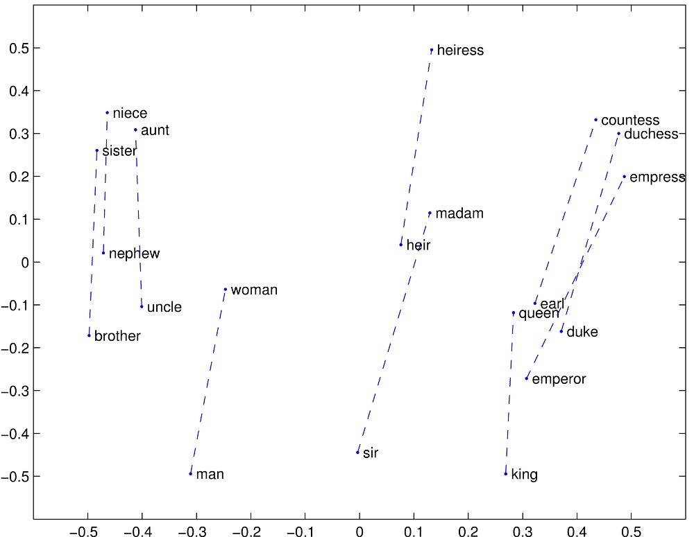
I remember the first time I heard about the magic of Deep Learning for Natural Language Processing (NLP). I was just starting a project with a young French startup Riminder and it was the first time I heard about word embeddings. There are moments in life when the confrontation with a new theory seems to make everything else irrelevant. Hearing about word vectors that encode similarity and meaning between words was one of these moments. I was baffled by the simplicity of the model as I started to play with these new concepts, building my first recurrent neural network for sentiment analysis. A few months later, as part of the master thesis of my master in the French university Ecole polytechnique I was working on more advanced models for sequence tagging at Proxem.
 |
Tensorflow vs Theano At that time, Tensorflow had just been open sourced and Theano was the most widely used framework. For those who are not familiar with the two, Theano operates at the matrix level while Tensorflow comes with a lot of pre-coded layers and helpful training mechanisms. Using Theano was sometimes painful but forced me to pay attention to the tiny details hidden in the equations and have a global understanding of how a deep learning library works.
Fastforward a few months: I’m in Stanford and I’m using Tensorflow. One day, here I am, asking myself: “What if you tried to code one of the sequence tagging models in Tensorflow? How long would it take?”. The answer is: no more than a few hours.
This post’s ambition is to provide an example of how to use Tensorflow to build a sate-of-the art model (similar to this paper) for sequence tagging and share some exciting NLP knowledge!
Together with this post, I am releasing the code and hope some will find it useful. You can use it to train your own sequence tagging model. I’ll assume conceptual knowledge about Recurrent Neural Networks. By the way, at this point I have to share my admiration for karpathy’s blog (and this post in particular “The Unreasonable Effectiveness of Recurrent Neural Networks”). For readers new to NLP, have a look at the amazing Stanford NLP class.
Task and Data
First, let’s discuss what Sequence Tagging is. Depending on your background, you may have heard of it under different names: Named Entity Recognition, Part-of-Speech Tagging, etc. We’ll focus on Named Entity Recognition (NER) for the rest of this post. You can check Wikipedia. One example is:
John  lives in New   York  and works for the European Union
B-PER O     O  B-LOC I-LOC O   O     O   O   B-ORG    I-ORG
In the CoNLL2003 task, the entities are LOC, PER, ORG and MISC for locations, persons, orgnizations and miscellaneous. The no-entity tag is O. Because some entities (like New York) have multiple words, we use a tagging scheme to distinguish between the beginning (tag B-...), or the inside of an entity (tag I-...). Other tagging schemes exist (IOBES, etc). However, if we just pause for a sec and think about it in an abstract manner, we just need a system that assigns a class (a number corresponding to a tag) to each word in a sentence.
“But wait, why is it a problem? Just keep a list of locations, common names and organizations!”
I am glad you asked this question. What makes this problem non-trivial is that a lot of entities, like names or organizations are just made-up names for which we don’t have any prior knowledge. Thus, what we really need is something that will extract contextual information from the sentence, just like humans do!
For our implementation, we are assuming that the data is stored in a .txt file with one word and its entity per line, like the following example
EU B-ORG
rejects O
German B-MISC
call O
to O
boycott O
British B-MISC
lamb O
. O

Peter B-PER
Blackburn I-PER
Model
“Let me guess… LSTM?”
You’re right. Like most of the NLP systems, ours is gonna rely on a recurrent neural network at some point. But before delving into the details of our model, let’s break it into 3 pieces:
- Word Representation: we need to use a dense representation $ w \in \mathbb{R}^n $ for each word. The first thing we can do is load some pre-trained word embeddings $ w_{glove} \in \mathbb{R}^{d_1} $ (GloVe, Word2Vec, Senna, etc.). We’re also going to extract some meaning from the characters. As we said, a lot of entities don’t even have a pretrained word vector, and the fact that the word starts with a capital letter may help for instance.
- Contextual Word Representation: for each word in its context, we need to get a meaningful representation $ h \in \mathbb{R}^k $. Good guess, we’re gonna use an LSTM here.
- Decoding: the ultimate step. Once we have a vector representing each word, we can use it to make a prediction.
Word Representation
For each word, we want to build a vector $ w \in \mathbb{R}^n $ that will capture the meaning and relevant features for our task. We’re gonna build this vector as a concatenation of the word embeddings $ w_{glove} \in \mathbb{R}^{d_1} $ from GloVe and a vector containing features extracted from the character level $ w_{chars} \in \mathbb{R}^{d_2} $. One option is to use hand-crafted features, like a component with a 0 or 1 if the word starts with a capital for instance. Another fancier option is to use some kind of neural network to make this extraction automatically for us. In this post, we’re gonna use a bi-LSTM at the character level, but we could use any other kind of recurrent neural network or even a convolutional neural network at the character or n-gram level.
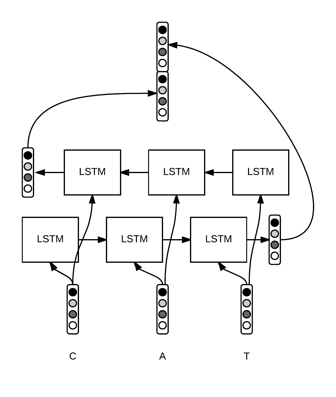 |
Each character $ c_i $ of a word $ w = [c_1, \ldots, c_p] $ (we make the distinction between lowercase and uppercase, for instance a and A are considered different) is associated to a vector $ c_i \in \mathbb{R}^{d_3} $. We run a bi-LSTM over the sequence of character embeddings and concatenate the final states to obtain a fixed-size vector $ w_{chars} \in \mathbb{R}^{d_2} $. Intuitively, this vector captures the morphology of the word. Then, we concatenate $ w_{chars} $ to the word embedding $ w_{glove} $ to get a vector representing our word $ w = [w_{glove}, w_{chars}] \in \mathbb{R}^n $ with $ n = d_1 + d_2 $.
Let’s have a look at the Tensorflow code. Recall that as Tensorflow receives batches of words and data, we need to pad sentences to make them the same length. As a result, we need to define 2 placeholders (= entries of the computational graph):
# shape = (batch size, max length of sentence in batch)
word_ids = tf.placeholder(tf.int32, shape=[None, None])

# shape = (batch size)
sequence_lengths = tf.placeholder(tf.int32, shape=[None])
Now, let’s use tensorflow built-in functions to load the word embeddings. Assume that embeddings is a numpy array with our GloVe embeddings, such that embeddings[i] gives the vector of the i-th word.
L = tf.Variable(embeddings, dtype=tf.float32, trainable=False)
# shape = (batch, sentence, word_vector_size)
pretrained_embeddings = tf.nn.embedding_lookup(L, word_ids)
You should use
tf.Variablewith argumenttrainable=Falseinstead oftf.constant, otherwise you risk memory issues!
Now, let’s build our representation from the characters. As we need to pad words to make them the same length, we also need to define 2 placeholders:
# shape = (batch size, max length of sentence, max length of word)
char_ids = tf.placeholder(tf.int32, shape=[None, None, None])

# shape = (batch_size, max_length of sentence)
word_lengths = tf.placeholder(tf.int32, shape=[None, None])
“Wait, can we use
Noneeverywhere like that? Why do we need it?”
Well, that’s up to us. It depends on how we perform our padding, but in this post we chose to do it dynamically, i.e. to pad to the maximum length in the batch. Thus, sentence length and word length will depend on the batch. Now, we can build the word embeddings from the characters. Here, we don’t have any pretrained character embeddings, so we call tf.get_variable that will initialize a matrix for us using the default initializer (xavier_initializer). We also need to reshape our 4-dimensional tensor to match the requirement of bidirectional_dynamic_rnn. Pay extra attention to the type returned by this function. Also, the state of the lstm is a tuple of memory and hidden state.
# 1. get character embeddings
K = tf.get_variable(name="char_embeddings", dtype=tf.float32,
    shape=[nchars, dim_char])
# shape = (batch, sentence, word, dim of char embeddings)
char_embeddings = tf.nn.embedding_lookup(K, char_ids)

# 2. put the time dimension on axis=1 for dynamic_rnn
s = tf.shape(char_embeddings) # store old shape
# shape = (batch x sentence, word, dim of char embeddings)
char_embeddings = tf.reshape(char_embeddings, shape=[-1, s[-2], s[-1]])
word_lengths = tf.reshape(self.word_lengths, shape=[-1])

# 3. bi lstm on chars
cell_fw = tf.contrib.rnn.LSTMCell(char_hidden_size, state_is_tuple=True)
cell_bw = tf.contrib.rnn.LSTMCell(char_hidden_size, state_is_tuple=True)

_, ((_, output_fw), (_, output_bw)) = tf.nn.bidirectional_dynamic_rnn(cell_fw,
    cell_bw, char_embeddings, sequence_length=word_lengths,
    dtype=tf.float32)
# shape = (batch x sentence, 2 x char_hidden_size)
output = tf.concat([output_fw, output_bw], axis=-1)

# shape = (batch, sentence, 2 x char_hidden_size)
char_rep = tf.reshape(output, shape=[-1, s[1], 2*char_hidden_size])

# shape = (batch, sentence, 2 x char_hidden_size + word_vector_size)
word_embeddings = tf.concat([pretrained_embeddings, char_rep], axis=-1)
Note the use of the special argument
sequence_lengththat ensures that the last state that we get is the last valid state. Thanks to this argument, for the unvalid time steps, thedynamic_rnnpasses the state through and outputs a vector of zeros.
Contextual Word Representation
Once we have our word representation $ w $, we simply run a LSTM (or bi-LSTM) over the sequence of word vectors and obtain another sequence of vectors (the hidden states of the LSTM or the concatenation of the two hidden states in the case of a bi-LSTM), $ h \in \mathbb{R}^k $.
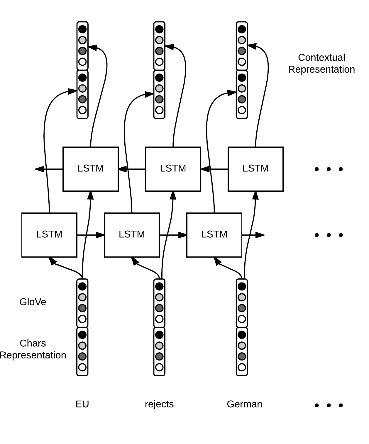 |
The tensorflow code is straightfoward. This time we use the hidden states of each time step and not just the final states. Thus, we had as input a sequence of $ m $ word vectors $ w_1, \ldots, w_m \in \mathbb{R}^n $ and now we have a sequence of vectors $ h_1, \ldots, h_m \in \mathbb{R}^k $. Whereas the $ w_t $ only captured information at the word level (syntax and semantics), the $ h_t $ also take context into account.
cell_fw = tf.contrib.rnn.LSTMCell(hidden_size)
cell_bw = tf.contrib.rnn.LSTMCell(hidden_size)

(output_fw, output_bw), _ = tf.nn.bidirectional_dynamic_rnn(cell_fw,
    cell_bw, word_embeddings, sequence_length=sequence_lengths,
    dtype=tf.float32)

context_rep = tf.concat([output_fw, output_bw], axis=-1)
Decoding
Computing Tags Scores At this stage, each word $ w $ is associated to a vector $ h $ that captures information from the meaning of the word, its characters and its context. Let’s use it to make a final prediction. We can use a fully connected neural network to get a vector where each entry corresponds to a score for each tag.
Let’s say we have $ 9 $ classes. We take a matrix $ W \in \mathbb{R}^{9 \times k} $ and $ b \in \mathbb{R}^9 $ and compute a vector of scores $ s \in \mathbb{R}^9 = W \cdot h + b $. We can interpret the $ i $-th component of $ s $ (that we will refer to as $ s[i] $) as the score of class $ i $ for word $ w $. One way to do this in tensorflow is:
W = tf.get_variable("W", shape=[2*self.config.hidden_size, self.config.ntags],
                dtype=tf.float32)

b = tf.get_variable("b", shape=[self.config.ntags], dtype=tf.float32,
                initializer=tf.zeros_initializer())

ntime_steps = tf.shape(context_rep)[1]
context_rep_flat = tf.reshape(context_rep, [-1, 2*hidden_size])
pred = tf.matmul(context_rep_flat, W) + b
scores = tf.reshape(pred, [-1, ntime_steps, ntags])
Note that we use a
zero_initializerfor the bias.
Decoding the scores Then, we have two options to make our final prediction.
In both cases, we want to be able to compute the probability $ \mathbb{P}(y_1, \ldots, y_m) $ of a tagging sequence $ y_t $ and find the sequence with the highest probability. Here, $ y_t $ is the id of the tag for the t-th word.
Here we have two options:
-
softmax: normalize the scores into a vector $ p \in \mathbb{R}^9 $ such that $ p[i]= \frac{e^{s[i]}}{\sum_{j=1}^9 e^{s[j]}} $. Then, $ p_i $ can be interpreted as the probability that the word belongs to class $ i $ (positive, sum to 1). Eventually, the probability $ \mathbb{P}(y) $ of a sequence of tag $ y $ is the product $ \prod_{t=1}^m p_t [y_t] $.
-
linear-chain CRF: the first method makes local choices. In other words, even if we capture some information from the context in our $ h $ thanks to the bi-LSTM, the tagging decision is still local. We don’t make use of the neighbooring tagging decisions. For instance, in
New York, the fact that we are taggingYorkas a location should help us to decide thatNewcorresponds to the beginning of a location. Given a sequence of words $ w_1, \ldots, w_m $, a sequence of score vectors $ s_1, \ldots, s_m $ and a sequence of tags $ y_1, \ldots, y_m $, a linear-chain CRF defines a global score $ C \in \mathbb{R} $ such that
where $ T $ is a transition matrix in $ \mathbb{R}^{9 \times 9} $ and $ e, b \in \mathbb{R}^9 $ are vectors of scores that capture the cost of beginning or ending with a given tag. The use of the matrix $ T $ captures linear (one step) dependencies between tagging decisions.
 |
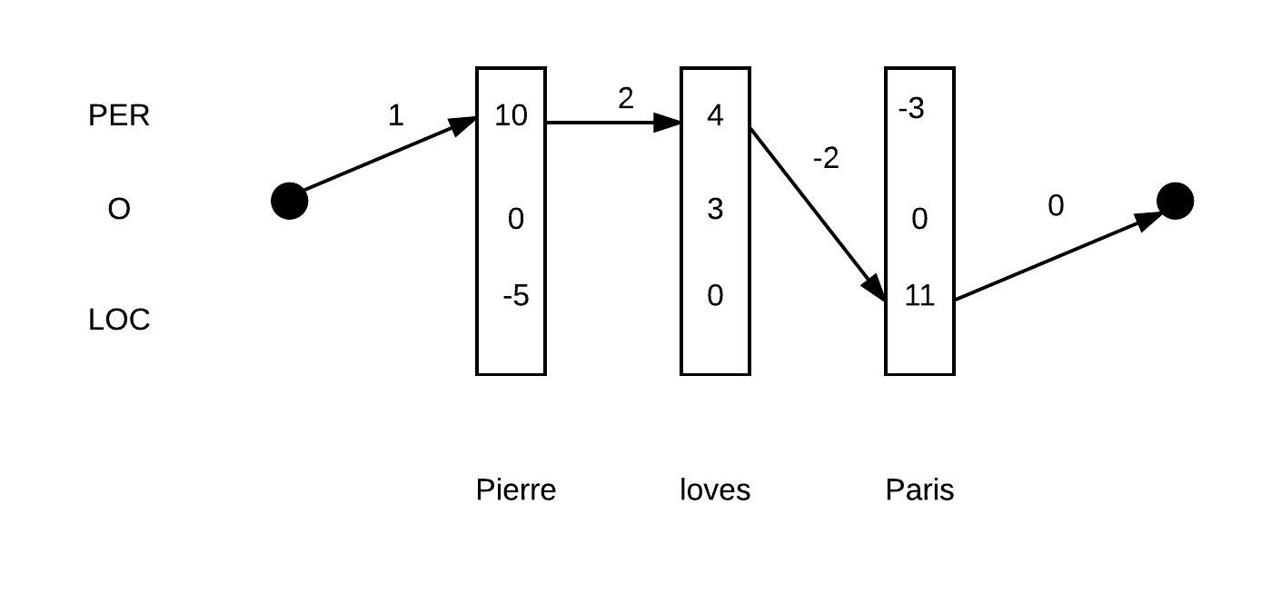 |
| The path PER-O-LOC has a score of $1+10+4+3+2+11+0=31$ | The path PER-PER-LOC has a score of $ 1+10+2+4-2+11+0=26 $ |
Now that we understand the scoring function of the CRF, we need to do 2 things:
- Find the sequence of tags with the best score.
- Compute a probability distribution over all the sequence of tags
“This sounds awesome, but don’t we have a computational problem as the number of possible tag choices is exponential?”
Finding the best sequence Well, you’re right. We cannot reasonnably imagine to compute the scores of all the $ 9^m $ tagging choices to choose the best one or even normalize each sequence score into a propability.
Luckily, the recurrent nature of our formula makes it the perfect candidate to apply dynamic programming. Let’s suppose that we have the solution $ \tilde{s}_{t+1} (y^{t+1}) $ for time steps $ t+1, \ldots, m $ for sequences that start with $ y^{t+1} $ for each of the 9 possible $ y^{t+1} $. Then, the solution $ \tilde{s}_t(y_t) $ for time steps $ t, \ldots, m $ that starts with $ y_t $ verifies
\[\begin{align*} \tilde{s}_t(y_t) &= \operatorname{argmax}_{y_t, \ldots, y_m} C(y_t, \ldots, y_m)\\ &= \operatorname{argmax}_{y_{t+1}} s_t [y_t] + T[y_{t}, y_{t+1}] + \tilde{s}_{t+1}(y^{t+1}) \end{align*}\]Then, each recurrence step is done in $ O(9 \times 9) $ (taking the argmax for each class). As we perform $ m $ steps, our final cost is $ O(9 \times 9 \times m) $ with is much better. For instance, for a sentence of 10 words we go from more than 3 billions ($ 9^{10} $) to just 810 in terms of complexity ( $ 9 \times 9 \times 10 )$!
Probability Distribution over the sequence of tags The final step of a linear chain CRF is to apply a softmax to the scores of all possible sequences to get the probabilty $ \mathbb{P}(y) $ of a given sequence of tags $ y $. To do that, we need to compute the partition factor
\[Z = \sum_{y_1, \ldots, y_m} e^{C(y_1, \ldots, y_m)}\]which is the sum of the scores of all possible sequences. We can apply the same idea as above, but instead of taking the argmax, we sum over all possible paths. Let’s call $ Z_t(y_t) $ the sum of scores for all sequences that start at time step $ t $ with tag $ y_t $. Then, $ Z_t $ verifies
\[\begin{align*} Z_t(y_t) &= \sum_{y_{t+1}} e^{s_t[y_t] + T[y_{t}, y_{t+1}]} \sum_{y_{t+2}, \ldots, y_m} e^{C(y_{t+1}, \ldots, y_m)} \\ &= \sum_{y_{t+1}} e^{s_t[y_t] + T[y_{t}, y_{t+1}]} \ Z_{t+1}(y_{t+1})\\ \log Z_t(y_t) &= \log \sum_{y_{t+1}} e^{s_t [y_t] + T[y_{t}, y_{t+1}] + \log Z_{t+1}(y_{t+1})} \end{align*}\]Then, we can easily define the probability of a given sequence of tags as
\[\mathbb{P}(y_1, \ldots, y_m) = \frac{e^{C(y_1, \ldots, y_m)}}{Z}\]Training
Now that we’ve explained the architecture of our model and spent some time on CRFs, a final word on our objective function. We are gonna use cross-entropy loss, in other words our loss is
\[- \log (\mathbb{P}(\tilde{y}))\]where $ \tilde{y} $ is the correct sequence of tags and its probability \(\mathbb{P}\) is given by
- CRF: $ \mathbb{P}(\tilde{y}) = \frac{e^{C(\tilde{y})}}{Z} $
- local softmax: $ \mathbb{P}(\tilde{y}) = \prod p_t[\tilde{y}^t] $.
“I’m afraid that coding the CRF loss is gonna be painful…”
Here comes the magic of open-source! Implementing a CRF only takes one-line! The following code computes the loss and also returns the matrix $ T $ (transition_params) that will be usefull for prediction.
# shape = (batch, sentence)
labels = tf.placeholder(tf.int32, shape=[None, None], name="labels")

log_likelihood, transition_params = tf.contrib.crf.crf_log_likelihood(
scores, labels, sequence_lengths)

loss = tf.reduce_mean(-log_likelihood)
In the case of the local softmax, the computation of the loss is more classic, but we have to pay extra attention to the padding and use tf.sequence_mask that transforms sequence lengths into boolean vectors (masks).
losses = tf.nn.sparse_softmax_cross_entropy_with_logits(logits=scores, labels=labels)
# shape = (batch, sentence, nclasses)
mask = tf.sequence_mask(sequence_lengths)
# apply mask
losses = tf.boolean_mask(losses, mask)

loss = tf.reduce_mean(losses)
And then, finally, we can define our train operator as
optimizer = tf.train.AdamOptimizer(self.lr)
train_op = optimizer.minimize(self.loss)
Using the trained model
For the local softmax method, performing the final prediction is straightfoward, the class is just the class with the highest score for each time step. This is done via tensorflow with :
labels_pred = tf.cast(tf.argmax(self.logits, axis=-1), tf.int32)
For the CRF, we have to use dynamic programming, as explained above. Again, this only take one line with tensorflow!
This function is pure ‘python’, as we get as argument the
transition_params. The tensorflowSession()evaluatesscore(= the $ s_t $ ), that’s all. Pay attention that this makes the prediction for only one sample!
The Viterbi decoding step is done in python for now, but as there seems to be some progress in contrib on similar problems (Beam Search for instance) we can hope for an ‘all-tensorflow’ CRF implementation anytime soon.
# shape = (sentence, nclasses)
score = ...
viterbi_sequence, viterbi_score = tf.contrib.crf.viterbi_decode(
                                score, transition_params)
With the previous code you should get an F1 score close between 90 and 91!
Conclusion
Tensorflow makes it really easy to implement any kind of deep learning system, as long as the layer you’re looking for is already implemented. However, you’ll still have to go to deeper levels if you’re trying something new…