Intro to tf.estimator and tf.data
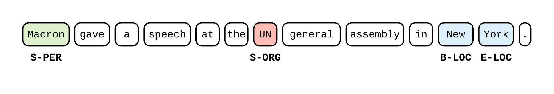
An example for Natural Language Processing (NER)
githubCode available on github.
Topics tf.data, tf.estimator, pathlib, LSTMBlockFusedCell, tf.contrib.lookup.index_table_from_file, tf.contrib.estimator.stop_if_no_increase_hook, tf.data.Dataset.from_generator, tf.metrics, tf.logging
Other
- You can find an overview of good practices of Tensorflow for NLP that I’ve written as part of my job as an NLP engineer at Roam Analytics (blog post, notebook, github)
- The course blog of Stanford’s CS230 also hosts some tutorials that I wrote with one of my friends, Olivier Moindrot.
This blog post provides an introduction to
tf.dataandtf.estimatorwith a step-by-step review of my bi-LSTM + CRF implementation.
Outline
- Introduction
- Global configuration
- Feed data with tf.data
- Define a model with tf.estimator
- Instantiate an Estimator
- Train an Estimator with early stopping
- Results and Conclusion
Introduction
Not so long ago, designing Deep Learning software meant writing custom Model classes. However, with code and implementations piling up on github and other open-source platforms, developers soon had enough examples to start designing unified high-level APIs for models and data loading. After all, we are all lazy and writing boilerplate code is not necessarily our cup of tea.
Thanks to intense competition on the Deep Learning Framework landscape, driving innovation and development of new functionnalities, brillant minds at Google and elsewhere worked on new additions to Tensorflow. Don’t ask me which version has it all (but I’m pretty sure 1.9 is good enough).
This blog post provides an example of how to use tf.data and tf.estimator for NLP and demonstrate how you can quickly get a state-of-the-art NLP model up and running with as few as a 100 lines of Tensorflow code!
Global configuration
If you like having an idea about what’s happening when you’re running your code, you need to change the level of verbosity of tensorflow logging (the module tf.logging which is built on top of the standard logging module). It does seem a bit weird that we have to take care of it, but hey, nothing is perfect and there probably is a reason that I am unaware of (nobody’s omniscient).
This snippet of code does a bit more than changing the verbosity: it also writes everything that tensorflow logs to a file. This is especially useful when you execute your code on a cluster of machines thanks to the help of a job manager (like slurm). The logs of stdout are probably accessible somewhere else, but I still think it’s better to have a version of it along with your weights and other stuff.
import logging
from pathlib import Path
import sys

import tensorflow as tf

# Setup logging
Path('results').mkdir(exist_ok=True)
tf.logging.set_verbosity(logging.INFO)
handlers = [
    logging.FileHandler('results/main.log'),
    logging.StreamHandler(sys.stdout)
]
logging.getLogger('tensorflow').handlers = handlers
If you don’t know / don’t use the
pathlibmodule (python3 only), try using it. It bundles a lot ofos.pathfunctionnality (and more) in a much nicer and easy-to-use package. I started using it after reading about it on this blog which also has a lot of other excellent articles.
We create two
handlers: one that will write the logs tosys.stdout(the terminal window so that you can see what’s going on), and one to a file (as theFileHandlername implies). I prefer resetting thehandlerscompletely to avoid double-logging.
So far, no Deep Learning, no Tensorflow (or barely), just python trickery.
Feed data with tf.data
When it comes to feeding data to your model (and to the tensorflow graph), there has been a few possible ways of achieving this in the past. The standard technique was to use a tf.placeholder that was updated through the run method of a tf.Session object. There was also an attempt of a more optimized input pipeline with threadings and queues.
Forget all this (first of all because we won’t use tf.Session anymore).
A better (and almost perfect) way of feeding data to your tensorflow model is to use a wonderful new tensorflow API called tf.data (thanks to the efforts of Derek Murray and others) whose philosophy, in a few words, is to create a special node of the graph that knows how to iterate the data and yield batches of tensors.
There is a bunch of official tutorials that you can find on the official website - something alas quite unusual. Here is a (short) selection:
- The official guide - Importing Data
- How to use
tf.data.Datasetwith the high level model APItf.estimator - The Neural Machine Translation Tutorial - A good example for NLP
A simple example
I am a great fan of the flexibility provided by tf.data.Dataset.from_generator. It allows you to do the data loading (from file or elsewhere) and some preprocessing in python before feeding it into the graph. Basically, defining such a dataset is just wiring the outputs of any python generator into Tensorflow Tensors.
Let’s define a dummy data generator
def generator_fn():
    for digit in range(2):
        line = 'I am digit {}'.format(digit)
        words = line.split()
        yield [w.encode() for w in words], len(words)
which yields
for words in generator_fn():
    print(words)
>>> ([b'I', b'am', b'digit', b'0'], 4)
>>> ([b'I', b'am', b'digit', b'1'], 4)
Good to know: when feeding string objects to your graph, you need to encode your string to
bytes.
Now, we want to make the output of this generator available inside our graph. Let’s create a special Dataset node
shapes = ([None], ())
types = (tf.string, tf.int32)

dataset = tf.data.Dataset.from_generator(generator_fn,
    output_shapes=shapes, output_types=types)
Tensorflow provides other ways of creating datasets, from text files (see
tf.data.TextLineDataset), from np arrays (seetf.data.Dataset.from_tensor_slices, from TF records (seetf.data.TFRecordDataset), etc. For most NLP cases, I advise you to take advantage of the flexibility given bytf.data.from_generatorunless you need the extra boost in performance provided by the other fancier options.
Test your tf.data pipeline
It is necessary to test that your
tf.datapipeline works as expected to avoid long hours of unnecessary headache and debugging.
There are 2 techniques to test your dataset.
-
Use the new
eager_executionmodeimport tensorflow as tf tf.enable_eager_execution() for tf_words, tf_size in dataset: print(tf_words, tf_size) >>> tf.Tensor([b'I' b'am' b'digit' b'0'], shape=(4,), dtype=string) tf.Tensor(4, shape=(), dtype=int32) >>> tf.Tensor([b'I' b'am' b'digit' b'1'], shape=(4,), dtype=string) tf.Tensor(4, shape=(), dtype=int32)The
tf.enable_eager_execution()must be called at program startup, just after yourimport tensorflow as tf -
Use an old-school, not-so-user-friendly-but-still-usefull
tf.Session. Before that, we need to create aniteratorout of our dataset. In other words, a dataset is an object that can be iterated, but we need to get the node created when iterating the dataset in order to evaluate it explicitely via aSession.iterator = dataset.make_one_shot_iterator() node = iterator.get_next() with tf.Session() as sess: print(sess.run(node)) print(sess.run(node)) # Each call moves the iterator to its next position >>> (array([b'I', b'am', b'digit', b'0'], dtype=object), 4) >>> (array([b'I', b'am', b'digit', b'1'], dtype=object), 4)print(node)sums up the above explanation in tensorflow-ic jargon - though a bit abstruse(<tf.Tensor 'IteratorGetNext_1:0' shape=(?,) dtype=string>, <tf.Tensor 'IteratorGetNext_1:1' shape=() dtype=int32>)
Read from file and tokenize
Now, a more complete example. We have 2 files words and tags, each line containing a white-spaced tokenized tagged sentence.
-
The generator function, that reads the files and parse the lines
 def parse_fn(line_words, line_tags):
     # Encode in Bytes for TF
     words = [w.encode() for w in line_words.strip().split()]
     tags = [t.encode() for t in line_tags.strip().split()]
     assert len(words) == len(tags), "Words and tags lengths don't match"
     return (words, len(words)), tags


 def generator_fn(words, tags):
     with Path(words).open('r') as f_words, Path(tags).open('r') as f_tags:
         for line_words, line_tags in zip(f_words, f_tags):
             yield parse_fn(line_words, line_tags)
Again, notice how we encode strings into
bytes -
The
input_fnthat constructs the dataset (we will need this function to work withtf.estimatorlater on)def input_fn(words, tags, params=None, shuffle_and_repeat=False): params = params if params is not None else {} shapes = (([None], ()), [None]) types = ((tf.string, tf.int32), tf.string) defaults = (('<pad>', 0), 'O') dataset = tf.data.Dataset.from_generator( functools.partial(generator_fn, words, tags), output_shapes=shapes, output_types=types) if shuffle_and_repeat: dataset = dataset.shuffle(params['buffer']).repeat(params['epochs']) dataset = (dataset .padded_batch(params.get('batch_size', 20), shapes, defaults) .prefetch(1)) return datasetNotice how we perform a few operations on our
datasetlikeshuffle,repeat,padded_batchandprefetch. These operations are self-explanatory, except maybe forprefetchwhich ensures that a batch of data is pre-loaded on the computing device so that it does not suffer from data starvation (= wasting compute resources that have to wait for the data to be transfered, a problem that occurs with GPUs and low compute / data ratios)Also be aware of the order of these operations. We want to
shufflebefore repeating (so that we shuffle inside one epoch = one full pass on the dataset). We then apply batching and the very final step is to prefetch.
We don’t forget to try out our new pipeline. Let’s create 2 files
words.txtI live in San Francisco You live in Paristags.txtO O O B-LOC I-LOC O O O S-LOC
And run the following code
dataset = input_fn('words.txt', 'tags.txt')
iterator = dataset.make_one_shot_iterator()
node = iterator.get_next()
with tf.Session() as sess:
    print(sess.run(node))
>>> ((array([[b'I', b'live', b'in', b'San', b'Francisco'],
>>>          [b'You', b'live', b'in', b'Paris', b'<pad>']],
>>>         dtype=object),
>>>   array([5, 4], dtype=int32)),
>>>   array([[b'O', b'O', b'O', b'B-LOC', b'I-LOC'],
>>>          [b'O', b'O', b'O', b'S-LOC', b'O']],
>>>          dtype=object))
As you can see, the
padded_batchworked as desired, by adding new tokens to the shorter sentence. Now, we have a batch of data which is ready to be consumed by our model!
Define a model with tf.estimator
Now let’s briefly give an overview of the tf.estimator paradigm. It consists of a high-level class tf.estimator.Estimator that provides all the useful training / evaluation / predict methods and handles weight serialization, Tensorboard etc. for you. To get such an instance, you need to define two components:
- A
model_fn(features, labels, mode, params) -> tf.estimator.EstimatorSpecwhose signature is strict and will hold the graph definition.featuresandlabelsare tensors (possibly nested structure of tensors, meaning tuples or dictionnaries)modeis a string, set by the Estimator. We will use this to specialize ourmodel_fndepending on the mode (PREDICT, EVAL or TRAIN).paramsis a dictionnary that will contain all our hyperparameters.
- An
input_fn(as the one we defined above) that returns atf.data.Dataset, which yields thefeaturesandlabelsconsumed by themodel_fn.
What if I need to manually set my features and labels?
The input_fn can also directly return the “nodes” obtained after iterating the dataset. This can be handy if you want to manually create your features as a dictionnary, or manually set labels to None in the case of a predict_input_fn for example. You would add these few lines at the end of the input_fn:
iterator = dataset.make_one_shot_iterator()
(words, nwords), tags = iterator.get_next()
features = {'words': words, 'nwords': words}
labels = {'tags': tags}  # Could be None in your predict_input_fn
return features, labels
Global Logic of the model_fn
The global design of the model_fn is straightforward, with no boilerplate code:
def model_fn(features, labels, mode, params):
    # Define the inference graph
    graph_outputs = some_tensorflow_applied_to(features)

    if mode == tf.estimator.ModeKeys.PREDICT:
        # Extract the predictions
        predictions = some_dict_from(graph_outputs)
        return tf.estimator.EstimatorSpec(mode, predictions=predictions)
    else:
        # Compute loss, metrics, tensorboard summaries
        loss = compute_loss_from(graph_outputs, labels)
        metrics = compute_metrics_from(graph_outputs, labels)

        if mode == tf.estimator.ModeKeys.EVAL:
            return tf.estimator.EstimatorSpec(
                mode, loss=loss, eval_metric_ops=metrics)

        elif mode == tf.estimator.ModeKeys.TRAIN:
            # Get train operator
            train_op = compute_train_op_from(graph_outputs, labels)
            return tf.estimator.EstimatorSpec(
                mode, loss=loss, train_op=train_op)

        else:
            raise NotImplementedError('Unknown mode {}'.format(mode))
Notice the hierarchisation and how each node is defined after an other, depending on the
mode.
And that’s all you need to define!
You can read the next part to get some details about our specific model and how we add metrics etc. If you want to know how to combine the model_fn with the input_fn, jump to the last part!
Define a bi-LSTM + CRF model_fn
Let’s implement a bi-LSTM + CRF for sequence tagging (Named Entity Recognition is one application) as defined in one of my other blog posts. Here is a step-by-step of the different blocks of our model_fn.
 |
You can find the full implementation here.
Parameters and vocabulary tables
Let’s extract and define a few variables at the beginning of our model_fn for easier reuse later on.
Nothing spectacular here, except that we use a tf.contrib.lookup.index_table_from_file that maps strings to ids in the Tensorflow graph.
dropout = params['dropout']
words, nwords = features
training = (mode == tf.estimator.ModeKeys.TRAIN)
vocab_words = tf.contrib.lookup.index_table_from_file(
    params['words'], num_oov_buckets=1)
with Path(params['tags']).open() as f:
    indices = [idx for idx, tag in enumerate(f) if tag.strip() != 'O']
    num_tags = len(indices) + 1
Here,
params['words']is the path to a file containing one lexeme (= an element of my vocabulary) per line. I use Tensorflow built-int lookup tables to map token strings to lexemes ids. We also use the same convention to store the vocabulary oftags.
Word Embeddings
The first step in our graph is getting the word representation.
- Use the Tensorflow vocabulary lookup table to map token strings to ids.
- Reload a
np.arraycontaining some pre-trained vectors (like GloVe) where the row index corresponds to a lexeme id. - Perform a lookup in this array to get the embedding of every token
- Apply dropout to the dense representation to prevent overfitting
word_ids = vocab_words.lookup(words)
glove = np.load(params['glove'])['embeddings']  # np.array
variable = np.vstack([glove, [[0.]*params['dim']]])  # For unknown words
variable = tf.Variable(variable, dtype=tf.float32, trainable=False)
embeddings = tf.nn.embedding_lookup(variable, word_ids)
embeddings = tf.layers.dropout(embeddings, rate=dropout, training=training)
Because some words might be absent from the vocabulary, we defined a non-zero
num_oov_bucketsin our vocabulary lookup table, which reserves new ids for unknown tokens. This means that we have to add new vectors for this ids at the end of our array of pre-trained embeddings.
Efficient bi-LSTM with LSTMBlockFusedCell
The second step is getting the context representation by applying a bi-LSTM on top of the token representation.
We use the most efficient implementation of the LSTM cell that combines all the LSTM operations (including recursion) in one CUDA kernel (at least that’s what I think is happening here).
This
LSTMBlockFusedCelloperates on the entire time sequence (no need to perform any recursion on our side like atf.nn.bidirectional_dynamic_rnncall). However, it requires a Tensor of shape[time_len x batch_size x input_size]which means we have to transpose ourembeddingstensor to be time-major.
t = tf.transpose(embeddings, perm=[1, 0, 2])  # Make time-major
lstm_cell_fw = tf.contrib.rnn.LSTMBlockFusedCell(params['lstm_size'])
lstm_cell_bw = tf.contrib.rnn.LSTMBlockFusedCell(params['lstm_size'])
lstm_cell_bw = tf.contrib.rnn.TimeReversedFusedRNN(lstm_cell_bw)
output_fw, _ = lstm_cell_fw(t, dtype=tf.float32, sequence_length=nwords)
output_bw, _ = lstm_cell_bw(t, dtype=tf.float32, sequence_length=nwords)
output = tf.concat([output_fw, output_bw], axis=-1)
output = tf.transpose(output, perm=[1, 0, 2])  # Make batch-major
output = tf.layers.dropout(output, rate=dropout, training=training)
Tensorflow CRF
The third step is decoding the sentence using a CRF.
We need to define our crf_params variable ourselves because we will need it to compute the CRF loss reusing the same parameters later on.
logits = tf.layers.dense(output, num_tags)
crf_params = tf.get_variable("crf", [num_tags, num_tags], dtype=tf.float32)
pred_ids, _ = tf.contrib.crf.crf_decode(logits, crf_params, nwords)
Now we’ve defined our graph outputs. Let’s cover the rest of the
model_fn.
PREDICT Mode
We create a reverse table to map the predicted tag ids back to tag strings and bundle our graph outputs into a predictions dictionary. It is important to notice here that the EstimatorSpec of the PREDICT mode only has tensors that depend on features. We haven’t used the labels so far (we will for the EVAL and TRAIN mode though).
if mode == tf.estimator.ModeKeys.PREDICT:
    # Predictions
    reverse_vocab_tags = tf.contrib.lookup.index_to_string_table_from_file(
        params['tags'])
    pred_strings = reverse_vocab_tags.lookup(tf.to_int64(pred_ids))
    predictions = {
        'pred_ids': pred_ids,
        'tags': pred_strings
    }
    return tf.estimator.EstimatorSpec(mode, predictions=predictions)
Loss for EVAL and TRAIN modes
We re-use our crf_params defined above to get the CRF loss and, again, use an index_table_from_file to map the tag strings to tag ids.
vocab_tags = tf.contrib.lookup.index_table_from_file(params['tags'])
tags = vocab_tags.lookup(labels)
log_likelihood, _ = tf.contrib.crf.crf_log_likelihood(
    logits, tags, nwords, crf_params)
loss = tf.reduce_mean(-log_likelihood)
Metrics and Tensorboard
We use one of my other projects, tf_metrics to get the micro average of multiclass classification metrics like precision, recall and f1, in the same way as scikit-learn does it. This allows us to treat the special null class O as a proper null class and get a global score of our model’s performance (at the token level).
import tf_metrics

# Metrics
weights = tf.sequence_mask(nwords)
metrics = {
    'acc': tf.metrics.accuracy(tags, pred_ids, weights),
    'precision': tf_metrics.precision(tags, pred_ids, num_tags, indices, weights),
    'recall': tf_metrics.recall(tags, pred_ids, num_tags, indices, weights),
    'f1': tf_metrics.f1(tags, pred_ids, num_tags, indices, weights),
}
# Tensoboard summaries
for metric_name, op in metrics.items():
    tf.summary.scalar(metric_name, op[1])
You can install tf_metrics with
pip install git+https://github.com/guillaumegenthial/tf_metrics.git
EVAL and TRAIN modes
Now that everything is setup, it is easy to define our EstimatorSpec for the EVAL and TRAIN modes.
if mode == tf.estimator.ModeKeys.EVAL:
    return tf.estimator.EstimatorSpec(
        mode, loss=loss, eval_metric_ops=metrics)

elif mode == tf.estimator.ModeKeys.TRAIN:
    train_op = tf.train.AdamOptimizer().minimize(
        loss, global_step=tf.train.get_or_create_global_step())
    return tf.estimator.EstimatorSpec(
        mode, loss=loss, train_op=train_op)
Instantiate an Estimator
Initializing our model is just a few lines of codes. As expected, we just need to provide the model_fn and some extra configuration.
# Params
params = {
    'dim': 300,
    'dropout': 0.5,
    'num_oov_buckets': 1,
    'epochs': 25,
    'batch_size': 20,
    'buffer': 15000,
    'lstm_size': 100,
    'words': str(Path(DATADIR, 'vocab.words.txt')),
    'chars': str(Path(DATADIR, 'vocab.chars.txt')),
    'tags': str(Path(DATADIR, 'vocab.tags.txt')),
    'glove': str(Path(DATADIR, 'glove.npz'))
}
cfg = tf.estimator.RunConfig(save_checkpoints_secs=120)
estimator = tf.estimator.Estimator(model_fn, 'results/model', cfg, params)
save_checkpoints_secs=120means that every 2 minutes (120 seconds) we want to serialize our weights to disk.
Train an Estimator with early stopping
Now that we have our estimator, we need to perform 3 steps
- Fully define our
input_fnon our different datasets. Because thetf.estimatorAPI expects callables, we use the standardfunctoolslibrary to provide parameters upon execution - We want to train our Estimator as long as our f1 score keeps improving (early-stopping). A way of achieving this is to use a
stop_if_no_increase_hook. Because the hook somehow assumes that the model’seval_dirhas already been created when it is first called (which is not always the case with our RunConfig), let’s make sure that theeval_direxists before even running our training. - Finally, run our training with the
train_and_evaluate. This method has recently been updated and does not destroy / re-create the graph each time we switch from training to evaluation and vice versa, which results in a very fast and efficient training process with automated evaluation on the development set once in a while! It also supports more advanced uses, like distributed training and evaluation etc. (out of the scope of this post).
# 1. Define our input_fn
train_inpf = functools.partial(input_fn, 'words.train.txt', 'tags.train.txt',
                               params, shuffle_and_repeat=True)
eval_inpf = functools.partial(input_fn,'words.testa.txt', 'tags.testa.txt'
                              params)

# 2. Create a hook
Path(estimator.eval_dir()).mkdir(parents=True, exist_ok=True)
hook = tf.contrib.estimator.stop_if_no_increase_hook(
    estimator, 'f1', 500, min_steps=8000, run_every_secs=120)
train_spec = tf.estimator.TrainSpec(input_fn=input_fn, hooks=[hook])
eval_spec = tf.estimator.EvalSpec(input_fn=eval_inpf, throttle_secs=120)

# 3. Train with early stopping
tf.estimator.train_and_evaluate(estimator, train_spec, eval_spec)
and now you should see appear stuff like
Running training and evaluation locally (non-distributed).
Start train and evaluate loop. The evaluate will happen after every checkpoint. Checkpoint frequency is determined based on RunConfig arguments: save_checkpoints_steps None or save_checkpoints_secs 60.
Calling model_fn.
Done calling model_fn.
Create CheckpointSaverHook.
Graph was finalized.
Running local_init_op.
Done running local_init_op.
Saving checkpoints for 0 into results/model/model.ckpt.
loss = 50.51557, step = 1
global_step/sec: 12.9584
loss = 5.384676, step = 101 (7.717 sec)
global_step/sec: 11.2308
loss = 2.8501458, step = 401 (8.903 sec)
global_step/sec: 12.725
Saving checkpoints for 688 into results/model/model.ckpt.
Calling model_fn.
Done calling model_fn.
Starting evaluation at 2018-09-09-22:24:21
Graph was finalized.
Restoring parameters from results/model/model.ckpt-688
Running local_init_op.
Done running local_init_op.
Finished evaluation at 2018-09-09-22:24:26
Saving dict for global step 688: acc = 0.972764, f1 = 0.8747083, global_step = 688, loss = 1.543679, precision = 0.89365673, recall = 0.8565468
Saving 'checkpoint_path' summary for global step 688: results/model/model.ckpt-688
global_step/sec: 5.57122
loss = 1.5974493, step = 701 (17.949 sec)
Results and Conclusion
You will find the complete implementation on github as well as other variants (with character embeddings, with Exponential Moving Average of weights, etc.).
For those curious about the results yielded by this implementation, I’ve conducted a few experiments on the CoNLL2003 dataset, training on train only with early stopping on testa and reported average, standard deviation and best of 5 runs. To compare with the results to the paper Bidirectional LSTM-CRF Models for Sequence Tagging by Huang, Xu and Yu.
Training time ~ 20 min on my laptop.
train |
testa |
testb |
Paper, testb |
|
|---|---|---|---|---|
| best | 98.45 | 93.81 | 90.61 | 90.10 |
| best (EMA) | 98.82 | 94.06 | 90.43 | |
| mean ± std | 98.85 ± 0.22 | 93.68 ± 0.12 | 90.42 ± 0.10 | |
| mean ± std (EMA) | 98.71 ± 0.47 | 93.81 ± 0.24 | 90.50 ± 0.21 | |
| abs. best | 90.61 | |||
| abs. best (EMA) | 90.75 |
If you enjoyed and want to contribute and suggest improvements, comments / PR / issues are welcome!